Building a network
Contents
Building a network
In the previous section, we have explained how reliable protocols allow hosts to exchange data reliably even if the underlying physical layer is imperfect and thus unreliable. Connecting two hosts together through a wire is the first step to build a network. However, this is not sufficient. Hosts usually need to interact with other hosts that are not directly connected through a direct physical layer link. This can be achieved by adding one layer above the datalink layer: the network layer.
The main objective of the network layer is to allow hosts, connected to different networks, to exchange information through intermediate systems called router. The unit of information in the network layer is called a packet.
Before explaining the operation of the network layer, it is useful to remember the characteristics of the service provided by the datalink layer. There are many variants of the datalink layer. Some provide a reliable service while others do not provide any guarantee of delivery. The reliable datalink layer services are popular in environments such as wireless networks where transmission errors are frequent. On the other hand, unreliable services are usually used when the physical layer provides an almost reliable service (i.e. only a negligible fraction of the frames are affected by transmission errors). Such almost reliable services are frequently used in wired and optical networks. In this chapter, we will assume that the datalink layer service provides an almost reliable service since this is both the most general one and also the most widely deployed one.
The point-to-point datalink layer

There are two main types of datalink layers. The simplest datalink layer is when there are only two communicating systems that are directly connected through the physical layer. Such a datalink layer is used when there is a point-to-point link between the two communicating systems. These two systems can be hosts or routers. PPP (Point-to-Point Protocol), defined in RFC 1661, is an example of such a point-to-point datalink layer. Datalink layer entities exchange frames. A datalink frame sent by a datalink layer entity on the left is transmitted through the physical layer, so that it can reach the datalink layer entity on the right. Point-to-point datalink layers can either provide an unreliable service (frames can be corrupted or lost) or a reliable service (in this case, the datalink layer includes retransmission mechanisms).
The second type of datalink layer is the one used in Local Area Networks (LAN). Conceptually, a LAN is a set of communicating devices such that any two devices can directly exchange frames through the datalink layer. Both hosts and routers can be connected to a LAN. Some LANs only connect a few devices, but there are LANs that can connect hundreds or even thousands of devices. In this chapter, we focus on the utilization of point-to-point datalink layers. We describe later the organization and the operation of Local Area Networks and their impact on the network layer.
Even if we only consider the point-to-point datalink layers, there is an important characteristic of these layers that we cannot ignore. No datalink layer is able to send frames of unlimited size. Each datalink layer is characterized by a maximum frame size. There are more than dozen different datalink layers and unfortunately most of them use a different maximum frame size. This heterogeneity in the maximum frame sizes will cause problems when we will need to exchange data between hosts attached to different types of datalink layers.
As a first step, let us assume that we only need to exchange a small amount of data. In this case, there is no issue with the maximum length of the frames. However, there are other more interesting problems that we need to tackle. To understand these problems, let us consider the network represented in the figure below.
A simple network containing three hosts and five routers

This network contains two types of devices. The hosts, represented with circles and the routers, represented as boxes. A host is a device which is able to send and receive data for its own usage in contrast with routers that most of the time simply forward data towards their final destination. Routers have multiple links to neighboring routers or hosts. Hosts are usually attached via a single link to the network. Nowadays, with the growth of wireless networks, more and more hosts are equipped with several physical interfaces. These hosts are often called multihomed. Still, using several interfaces at the same time often leads to practical issues that are beyond the scope of this document. For this reason, we only consider single-homed hosts in this e-book.
To understand the key principles behind the operation of a network, let us analyze all the operations that need to be performed to allow host A in the above network to send one byte to host B. Thanks to the datalink layer used above the A-R1 link, host A can easily send a byte to router R1 inside a frame. However, upon reception of this frame, router R1 needs to understand that this byte is destined to host B and not to itself. This is the objective of the network layer.
The network layer enables the transmission of information between hosts that are not directly connected through intermediate routers. This transmission is carried out by putting the information to be transmitted inside a data structure which is called a packet. As a frame that contains useful data and control information, a packet also contains both data supplied by the user and control information. An important issue in the network layer is the ability to identify a node (host or router) inside the network. This identification is performed by associating an address to each node. An address is usually represented as a sequence of bits. Most networks use fixed-length addresses. At this stage, let us simply assume that each of the nodes in the above network has an address which corresponds to the binary representation of its name on the figure.
To send one byte of information to host B, host A needs to place this information inside a packet. In addition to the data being transmitted, the packet also contains either the addresses of the source and the destination nodes or information that indicates the path that needs to be followed to reach the destination.
There are two possible organizations for the network layer :
datagram
virtual circuits
The datagram organization
The first and most popular organization of the network layer is the datagram organization. This organization is inspired by the organization of the postal service. Each host is identified by a network layer address. To send information to a remote host, a host creates a packet that contains:
the network layer address of the destination host
its own network layer address
the information to be sent
To understand the datagram organization, let us consider the figure below. A network layer address, represented by a letter, has been assigned to each host and router. To send some information to host J, host A creates a packet containing its own address, the destination address and the information to be exchanged.
A simple internetwork
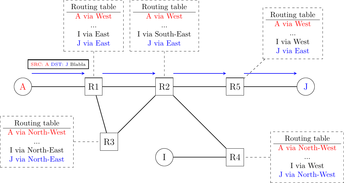
With the datagram organization, routers use hop-by-hop forwarding. This means that when a router receives a packet that is not destined to itself, it looks up the destination address of the packet in its forwarding table. A forwarding table is a data structure that maps each destination address (or set of destination addresses) to the outgoing interface over which a packet destined to this address must be forwarded to reach its final destination. The router consults its forwarding table to forward each packet that it handles.
The figure illustrates some possible forwarding tables in this network. By inspecting the forwarding tables of the different routers, one can find the path followed by packets sent from a source to a particular destination. In the example above, host A sends its packet to router R1. R1 consults its forwarding table and forwards the packet towards R2. Based on its own table, R2 decides to forward the packet to R5 that can deliver it to its destination. Thus, the path from A to J is A -> R1 -> R2 -> R5 -> J.
The computation of the forwarding tables of all the routers inside a network is a key element for the correct operation of the network. This computation can be carried out by using either distributed or centralized algorithms. These algorithms provide different performance, may lead to different types of paths, but their composition must lead to valid paths.
In a network, a path can be defined as the list of all intermediate routers for a given source destination pair. For a given source/destination pair, the path can be derived by first consulting the forwarding table of the router attached to the source to determine the next router on the path towards the chosen destination. Then, the forwarding table of this router is queried for the same destination… The queries continue until the destination is reached. In a network that has valid forwarding tables, all the paths between all source/destination pairs contain a finite number of intermediate routers. However, if forwarding tables have not been correctly computed, two types of invalid paths can occur.
A path may lead to a black hole. In a network, a black hole is a router that receives packets for at least one given source/destination pair but does not have an entry inside its forwarding table for this destination. Since it does not know how to reach the destination, the router cannot forward the received packets and must discard them. Any centralized or distributed algorithm that computes forwarding tables must ensure that there are not black holes inside the network.
A second type of problem may exist in networks using the datagram organization. Consider a path that contains a cycle. For example, router R1 sends all packets towards destination D via router R2. Router R2 forwards these packets to router R3 and finally router R3’s forwarding table uses router R1 as its nexthop to reach destination D. In this case, if a packet destined to D is received by router R1, it will loop on the R1 -> R2 -> R3 -> R1 cycle and will never reach its final destination. As in the black hole case, the destination is not reachable from all sources in the network. In practice the loop problem is more annoying than the black hole problem because when a packet is caught in a forwarding loop, it unnecessarily consumes bandwidth. In the black hole case, the problematic packet is quickly discarded. We will see later that network layer protocols include techniques to minimize the impact of such forwarding loops.
Any solution which is used to compute the forwarding tables of a network must ensure that all destinations are reachable from any source. This implies that it must guarantee the absence of black holes and forwarding loops.
The forwarding tables and the precise format of the packets that are exchanged inside the network are part of the data plane of the network. This data plane contains all the protocols and algorithms that are used by hosts and routers to create and process the packets that contain user data. On high-end routers, the data plane is often implemented in hardware for performance reasons.
Besides the data plane, a network is also characterized by its control plane. The control plane includes all the protocols and algorithms (often distributed) that compute the forwarding tables that are installed on all routers inside the network. While there is only one possible data plane for a given networking technology, different networks using the same technology may use different control planes.
The simplest control plane for a network is to manually compute the forwarding tables of all routers inside the network. This simple control plane is sufficient when the network is (very) small, usually up to a few routers.
In most networks, manual forwarding tables are not a solution for two reasons. First, most networks are too large to enable a manual computation of the forwarding tables. Second, with manually computed forwarding tables, it is very difficult to deal with link and router failures. Networks need to operate 24h a day, 365 days per year. Many events can affect the routers and links that compose a network. Link failures are regular events in deployed networks. Links can fail for various reasons, including electromagnetic interference, fiber cuts, hardware or software problems on the terminating routers,… Some links also need to be either added to or removed from the network because their utilization is too low or their cost is too high.
Similarly, routers also fail. There are two types of failures that affect routers. A router may stop forwarding packets due to hardware or software problems (e.g., due to a crash of its operating system). A router may also need to be halted from time to time (e.g., to upgrade its operating system or to install new interface cards). These planned and unplanned events affect the set of links and routers that can be used to forward packets in the network. Still, most network users expect that their network will continue to correctly forward packets despite all these events. With manually computed forwarding tables, it is usually impossible to pre-compute the forwarding tables while taking into account all possible failure scenarios.
An alternative to manually computed forwarding tables is to use a network management platform that tracks the network status and can push new forwarding tables on the routers when it detects any modification to the network topology. This solution gives some flexibility to the network managers in computing the paths inside their network. However, this solution only works if the network management platform is always capable of reaching all routers even when the network topology changes. This may require a dedicated network that allows the management platform to push information on the forwarding tables. Openflow is a modern example of such solutions [MAB2008]. In a nutshell, Openflow is a protocol that enables a network controller to install specific entries in the forwarding tables of remote routers and much more.
Another interesting point that is worth being discussed is when the forwarding tables are computed. A widely used solution is to compute the entries of the forwarding tables for all destinations on all routers. This ensures that each router has a valid route towards each destination. These entries can be updated when an event occurs and the network topology changes. A drawback of this approach is that the forwarding tables can become large in large networks since each router must always maintain one entry for each destination inside its forwarding table.
Some networks use the arrival of packets as the trigger to compute the corresponding entries in the forwarding tables. Several technologies have been built upon this principle. When a packet arrives, the router consults its forwarding table to find a path towards the destination. If the destination is present in the forwarding table, the packet is forwarded. Otherwise, the router needs to find a way to forward the packet and update its forwarding table.
Computing forwarding tables
Networks deployed several techniques to update the forwarding tables upon the arrival of a packet. In this section, we briefly present the principles that underlie three of these techniques.
The first technique assumes that the underlying network topology is a tree. A tree is the simplest network to be considered when forwarding packets. The main advantage of using a tree is that there is only one path between any pair of nodes inside the network. Since a tree does not contain any cycle, it is impossible to have forwarding loops in a tree-shaped network.
In a tree-shaped network, it is relatively simple for each node to automatically compute its forwarding table by inspecting the packets that it receives. For this, each node uses the source and destination addresses present inside each packet. Thanks to the source address, a node can learn the location of the different sources inside the network. Each source has a unique address. When a node receives a packet over a given interface, it learns that the source (address) of this packet is reachable via this interface. The node maintains a data structure that maps each known source address to an incoming interface. This data structure is often called the port-address table since it indicates the interface (or port) to reach a given address.
Learning the location of the sources is not sufficient, nodes also need to forward packets towards their destination. When a node receives a packet whose destination address is already present inside its port-address table, it simply forwards the packet on the interface listed in the port-address table. In this case, the packet will follow the port-address table entries in the downstream nodes and will reach the destination. If the destination address is not included in the port-address table, the node simply forwards the packet on all its interfaces, except the interface from which the packet was received. Forwarding a packet over all interfaces is usually called broadcasting in the terminology of computer networks. Sending the packet over all interfaces except one is a costly operation since the packet is sent over links that do not reach the destination. Given the tree-shape of the network, the packet will explore all downstream branches of the tree and will finally reach its destination. In practice, the broadcasting operation does not occur too often and its performance impact remains limited.
To understand the operation of the port-address table, let us consider the example network shown in the figure below. This network contains three hosts: A, B and C and five routers, R1 to R5. When the network boots, all the forwarding tables of the nodes are empty.
A simple tree-shaped network
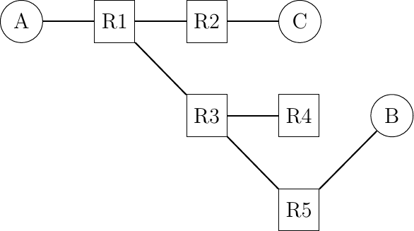
Host A sends a packet towards B. When receiving this packet, R1 learns that A is reachable via its West interface. Since it does not have an entry for destination B in its port-address table, it forwards the packet to both R2 and R3. When R2 receives the packet, it updates its own forwarding table and forward the packet to C. Since C is not the intended recipient, it simply discards the received packet. Router R3 also receives the packet. It learns that A is reachable via its North-West interface and broadcasts the packet to R4 and R5. R5 also updates its forwarding table and finally forwards it to destination B. Let us now consider what happens when B sends a reply to A. R5 first learns that B is attached to its North-East port. It then consults its port-address table and finds that A is reachable via its North-West interface. The packet is then forwarded hop-by-hop to A without any broadcasting. Later on, if C sends a packet to B, this packet will reach R1 that contains a valid forwarding entry in its forwarding table.
By inspecting the source and destination addresses of packets, network nodes can automatically derive their forwarding tables. As we will discuss later, this technique is used in Ethernet networks. Despite being widely used, it has two important drawbacks. First, packets sent to unknown destinations are broadcasted in the network even if the destination is not attached to the network. Consider the transmission of ten packets destined to Z in the network above. When a node receives a packet towards this destination, it can only broadcast that packet. Since Z is not attached to the network, no node will ever receive a packet whose source is Z to update its forwarding table. The second and more important problem is that few networks have a tree-shaped topology. It is interesting to analyze what happens when a port-address table is used in a network that contains a cycle. Consider the simple network shown below with a single host.
A simple and redundant network
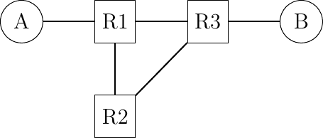
Assume that the network has started and all port-address and forwarding tables are empty. Host A sends a packet towards B. Upon reception of this packet, R1 updates its port-address table. Since B is not present in the port-address table, the packet is broadcasted. Both R2 and R3 receive a copy of the packet sent by A. They both update their port-address table. Unfortunately, they also both broadcast the received packet. B receives a first copy of the packet, but R3 and R2 receive it again. R3 will then broadcast this copy of the packet to B and R1 while R2 will broadcast its copy to R1. Although B has already received two copies of the packet, it is still inside the network and continues to loop. Due to the presence of the cycle, a single packet towards an unknown destination generates many copies of this packet that loop and will eventually saturate the network. Network operators who are using port-address tables to automatically compute the forwarding tables also use distributed algorithms to ensure that the network topology is always a tree.
Another technique called source routing can be used to automatically compute forwarding tables. It has been used in interconnecting Token Ring networks and in some wireless networks. Intuitively, source routing enables a destination to automatically discover the paths from a given source towards itself. This technique requires nodes to encode information inside some packets. For simplicity, let us assume that the data plane supports two types of packets :
the data packets
the control packets
Data packets are used to exchange data while control packets are used to discover the paths between hosts. With source routing, routers can be kept as simple as possible and all the complexity is placed on the hosts. This is in contrast with the previous technique where the nodes had to maintain a port-address and a forwarding table while the hosts simply sent and received packets. Each node is configured with one unique address and there is one identifier per outgoing link. For simplicity and to avoid cluttering the figures with those identifiers, we assume that each node uses as link identifiers north, west, south,… In practice, a node would associate one integer to each outgoing link.
A simple network with two hosts and four routers
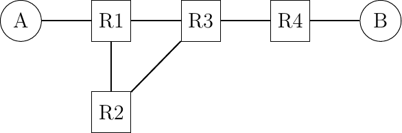
In the network above, router R2 is attached to two outgoing links. R2 is connected to both R1 and R3. R2 can easily determine that it is connected to these two nodes by exchanging packets with them or observing the packets that it receives over each interface. Assume for example that when a node (either host or router) starts, it sends a special control packet over each of its interfaces to advertise its own address to its neighbors. When a node receives such a packet, it automatically replies with its own address. This exchange can also be used to verify whether a neighbor, either router or host, is still alive. With source routing, the data plane packets include a list of identifiers. This list is called a source route. It indicates the path to be followed by the packet as a sequence of link identifiers. When a node receives such a data plane packet, it first checks whether the packet’s destination is a direct neighbor. In this case, the packet is forwarded to this neighbor. Otherwise, the node extracts the next address from the list and forwards it to the neighbor. This allows the source to specify the explicit path to be followed for each packet. For example, in the figure above there are two possible paths between A and B. To use the path via R2, A would send a packet that contains R1,R2,R3 as source route. To avoid going via R2, A would place R1,R3 as the source route in its transmitted packet. If A knows the complete network topology and all link identifiers, it can easily compute the source route towards each destination. It can even use different paths, e.g. for redundancy, to reach a given destination. However, in a real network hosts do not usually have a map of the entire network topology.
In networks that rely on source routing, hosts use control packets to automatically discover the best path(s). In addition to the source and destination addresses, control packets contain a list that records the intermediate nodes. This list is often called the record route because it allows recording the route followed by a given packet. When a node receives such a control packet, it first checks whether its address is included in the record route. If yes, the packet has already been forwarded by this node and it is silently discarded. Otherwise, it adds its own address to the record route and forwards the packet to all its interfaces, except the interface over which the packet has been received. Thanks to this, the control packet can explore all paths between a source and a given destination.
For example, consider again the network topology above. A sends a control packet towards B. The initial record route is empty. When R1 receives the packet, it adds its own address to the record route and forwards a copy to R2 and another to R3. R2 receives the packet, adds itself to the record route and forwards it to R3. R3 receives two copies of the packet. The first contains the [R1,R2] record route and the second [R1]. In the end, B will receive two control packets containing [R1,R2,R3,R4] and [R1,R3,R4] as record routes. B can keep these two paths or select the best one and discard the second. A popular heuristic is to select the record route of the first received packet as being the best one since this likely corresponds to the shortest delay path.
With the received record route, B can send a data packet to A. For this, it simply reverses the chosen record route. However, we still need to communicate the chosen path to A. This can be done by putting the record route inside a control packet which is sent back to A over the reverse path. An alternative is to simply send a data packet back to A. This packet will travel back to A. To allow A to inspect the entire path followed by the data packet, its source route must contain all intermediate routers when it is received by A. This can be achieved by encoding the source route using a data structure that contains an index and the ordered list of node addresses. The index always points to the next address in the source route. It is initialized at 0 when a packet is created and incremented by each intermediate node.
The third technique to compute forwarding tables is to rely on a control plane using a distributed algorithm. Routers exchange control messages to discover the network topology and build their forwarding table based on them. We dedicate a more detailed description of such distributed algorithms later in this section.
Flat or hierarchical addresses
The last, but important, point to discuss about the data plane of the networks that rely on the datagram mode is their addressing scheme. In the examples above, we have used letters to represent the addresses of the hosts and network nodes. In practice, all addresses are encoded as a bit string. Most network technologies use a fixed size bit string to represent source and destination address. These addresses can be organized in two different ways.
The first organization, which is the one that we have implicitly assumed until now, is the flat addressing scheme. Under this scheme, each host and network node has a unique address. The unicity of the addresses is important for the operation of the network. If two hosts have the same address, it can become difficult for the network to forward packets towards this destination. Flat addresses are typically used in situations where network nodes and hosts need to be able to communicate immediately with unique addresses. These flat addresses are often embedded inside the network interface cards. The network card manufacturer creates one unique address for each interface and this address is stored in the read-only memory of the interface. An advantage of this addressing scheme is that it easily supports unstructured and mobile networks. When a host moves, it can attach to another network and remain confident that its address is unique and enables it to communicate inside the new network.
With flat addressing the lookup operation in the forwarding table can be implemented as an exact match. The forwarding table contains the (sorted) list of all known destination addresses. When a packet arrives, a network node only needs to check whether this address is included in the forwarding table or not. In software, this is an O(log(n)) operation if the list is sorted. In hardware, Content Addressable Memories can efficiently perform this lookup operation, but their size is usually limited.
A drawback of the flat addressing scheme is that the forwarding tables linearly grow with the number of hosts and routers in the network. With this addressing scheme, each forwarding table must contain an entry that points to every address reachable inside the network. Since large networks can contain tens of millions of hosts or more, this is a major problem on routers that need to be able to quickly forward packets. As an illustration, it is interesting to consider the case of an interface running at 10 Gbps. Such interfaces are found on high-end servers and in various routers today. Assuming a packet size of 1000 bits, a pretty large and conservative number, such interface must forward ten million packets every second. This implies that a router that receives packets over such a link must forward one 1000 bits packet every 100 nanoseconds. This is the same order of magnitude as the memory access times of old DRAMs.
A widely used alternative to the flat addressing scheme is the hierarchical addressing scheme. This addressing scheme builds upon the fact that networks usually contain much more hosts than routers. In this case, a first solution to reduce the size of the forwarding tables is to create a hierarchy of addresses. This is the solution chosen by the post office since postal addresses contain a country, sometimes a state or province, a city, a street and finally a street number. When an envelope is forwarded by a post office in a remote country, it only looks at the destination country, while a post office in the same province will look at the city information. Only the post office responsible for a given city will look at the street name and only the postman will use the street number. Hierarchical addresses provide a similar solution for network addresses. For example, the address of an Internet host attached to a campus network could contain in the high-order bits an identification of the Internet Service Provider (ISP) that serves the campus network. Then, a subsequent block of bits identifies the campus network which is one of the customers of the ISP. Finally, the low order bits of the address identify the host in the campus network.
This hierarchical allocation of addresses can be applied in any type of network. In practice, the allocation of the addresses must follow the network topology. Usually, this is achieved by dividing the addressing space in consecutive blocks and then allocating these blocks to different parts of the network. In a small network, the simplest solution is to allocate one block of addresses to each network node and assign the host addresses from the attached node.
A simple network with two hosts and four routers
In the above figure, assume that the network uses 16 bits addresses and that the prefix 01001010 has been assigned to the entire network. Since the network contains four routers, the network operator could assign one block of sixty-four addresses to each router. R1 would use address 0100101000000000 while A could use address 0100101000000001. R2 could be assigned all addresses from 0100101001000000 to 0100101001111111. R4 could then use 0100101011000000 and assign 0100101011000001 to B. Other allocation schemes are possible. For example, R3 could be allocated a larger block of addresses than R2 and R4 could use a sub-block from R3 ‘s address block.
The main advantage of hierarchical addresses is that it is possible to significantly reduce the size of the forwarding tables. In many networks, the number of routers can be several orders of magnitude smaller than the number of hosts. A campus network may contain a dozen routers and thousands of hosts. The largest Internet Services Providers typically contain no more than a few tens of thousands of routers but still serve tens or hundreds of millions of hosts.
Despite their popularity, hierarchical addresses have some drawbacks. Their first drawback is that a lookup in the forwarding table is more complex than when using flat addresses. For example, on the Internet, network nodes have to perform a longest-match to forward each packet. This is partially compensated by the reduction in the size of the forwarding tables, but the additional complexity of the lookup operation has been a difficulty to implement hardware support for packet forwarding. A second drawback of the utilization of hierarchical addresses is that when a host connects for the first time to a network, it must contact one router to determine its own address. This requires some packet exchanges between the host and some routers. Furthermore, if a host moves and is attached to another routers, its network address will change. This can be an issue with some mobile hosts.
Dealing with heterogeneous datalink layers
Sometimes, the network layer needs to deal with heterogeneous datalink layers. For example, two hosts connected to different datalink layers exchange packets via routers that are using other types of datalink layers. Thanks to the network layer, this exchange of packets is possible provided that each packet can be placed inside a datalink layer frame before being transmitted. If all datalink layers support the same frame size, this is simple. When a node receives a frame, it decapsulates the packet that it contains, checks the header and forwards it, encapsulated inside another frame, to the outgoing interface. Unfortunately, the encapsulation operation is not always possible. Each datalink layer is characterized by the maximum frame size that it supports. Datalink layers typically support frames containing up to a few hundreds or a few thousands of bytes. The maximum frame size that a given datalink layer supports depends on its underlying technology. Unfortunately, most datalink layers support a different maximum frame size. This implies that when a host sends a large packet inside a frame to its nexthop router, there is a risk that this packet will have to traverse a link that is not capable of forwarding the packet inside a single frame. In principle, there are three possibilities to solve this problem. To discuss them, we consider a simple scenario with two hosts connected to a router as shown in the figure below.
A simple heterogeneous network

Consider in the network above that host A wants to send a 900 bytes packet (870 bytes of payload and 30 bytes of header) to host B via router R1. Host A encapsulates this packet inside a single frame. The frame is received by router R1 which extracts the packet. Router R1 has three possible options to process this packet.
The packet is too large and router R1 cannot forward it to router R2. It rejects the packet and sends a control packet back to the source (host A) to indicate that it cannot forward packets longer than 500 bytes (minus the packet header). The source could react to this control packet by retransmitting the information in smaller packets.
The network layer is able to fragment a packet. In our example, the router could fragment the packet in two parts. The first part contains the beginning of the payload and the second the end. There are two possible ways to perform this fragmentation.
Router R1 fragments the packet into two fragments before transmitting them to router R2. Router R2 reassembles the two packet fragments in a larger packet before transmitting them on the link towards host B.
Each of the packet fragments is a valid packet that contains a header with the source (host A) and destination (host B) addresses. When router R2 receives a packet fragment, it treats this packet as a regular packet and forwards it to its final destination (host B). Host B reassembles the received fragments.
These three solutions have advantages and drawbacks. With the first solution, routers remain simple and do not need to perform any fragmentation operation. This is important when routers are implemented mainly in hardware. However, hosts must be complex since they need to store the packets that they produce if they need to pass through a link that does not support large packets. This increases the buffering required on the hosts.
Furthermore, a single large packet may potentially need to be retransmitted several times. Consider for example a network similar to the one shown above but with four routers. Assume that the link R1->R2 supports 1000 bytes packets, link R2->R3 800 bytes packets and link R3->R4 600 bytes packets. A host attached to R1 that sends large packet will have to first try 1000 bytes, then 800 bytes and finally 600 bytes. Fortunately, this scenario does not occur very often in practice and this is the reason why this solution is used in real networks.
Fragmenting packets on a per-link basis, as presented for the second solution, can minimize the transmission overhead since a packet is only fragmented on the links where fragmentation is required. Large packets can continue to be used downstream of a link that only accepts small packets. However, this reduction of the overhead comes with two drawbacks. First, fragmenting packets, potentially on all links, increases the processing time and the buffer requirements on the routers. Second, this solution leads to a longer end-to-end delay since the downstream router has to reassemble all the packet fragments before forwarding the packet.
The last solution is a compromise between the two others. Routers need to perform fragmentation but they do not need to reassemble packet fragments. Only the hosts need to have buffers to reassemble the received fragments. This solution has a lower end-to-end delay and requires fewer processing time and memory on the routers.
The first solution to the fragmentation problem presented above suggests the utilization of control packets to inform the source about the reception of a too long packet. This is only one of the functions that are performed by the control protocol in the network layer. Other functions include :
sending a control packet back to the source if a packet is received by a router that does not have a valid entry in its forwarding table
sending a control packet back to the source if a router detects that a packet is looping inside the network
verifying that packets can reach a given destination
We will discuss these functions in more details when we will describe the protocols that are used in the network layer of the TCP/IP protocol suite.
Virtual circuit organization
The second organization of the network layer, called virtual circuits, has been inspired by the organization of telephone networks. Telephone networks have been designed to carry phone calls that usually last a few minutes. Each phone is identified by a telephone number and is attached to a telephone switch. To initiate a phone call, a telephone first needs to send the destination’s phone number to its local switch. The switch cooperates with the other switches in the network to create a bi-directional channel between the two telephones through the network. This channel will be used by the two telephones during the lifetime of the call and will be released at the end of the call. Until the 1960s, most of these channels were created manually, by telephone operators, upon request of the caller. Today’s telephone networks use automated switches and allow several channels to be carried over the same physical link, but the principles roughly remain the same.
In a network using virtual circuits, all hosts are also identified with a network layer address. However, packet forwarding is not performed by looking at the destination address of each packet. With the virtual circuit organization, each data packet contains one label 1. A label is an integer which is part of the packet header. Routers implement label switching to forward labelled data packet. Upon reception of a packet, a router consults its label forwarding table to find the outgoing interface for this packet. In contrast with the datagram mode, this lookup is very simple. The label forwarding table is an array stored in memory and the label of the incoming packet is the index to access this array. This implies that the lookup operation has an O(1) complexity in contrast with other packet forwarding techniques. To ensure that on each node the packet label is an index in the label forwarding table, each router that forwards a packet replaces the label of the forwarded packet with the label found in the label forwarding table. Each entry of the label forwarding table contains two pieces of information :
the outgoing interface for the packet
the label for the outgoing packet
For example, consider the label forwarding table of a network node below.
index |
outgoing interface |
label |
0 |
South |
7 |
1 |
none |
none |
2 |
West |
2 |
3 |
East |
2 |
If this node receives a packet with label=2, it forwards the packet on its West interface and sets the label of the outgoing packet to 2. If the received packet’s label is set to 3, then the packet is forwarded over the East interface and the label of the outgoing packet is set to 2. If a packet is received with a label field set to 1, the packet is discarded since the corresponding label forwarding table entry is invalid.
Label switching enables a full control over the path followed by packets inside the network. Consider the network below and assume that we want to use two virtual circuits : R1->R3->R4->R2->R5 and R2->R1->R3->R4->R5.
An example of network where label switching can be applied to tune its paths
To create these virtual circuits, we need to configure the label forwarding tables of all routers. For simplicity, assume that a label forwarding table only contains two entries. Assume that R5 wants to receive the packets from the virtual circuit created by R1 (resp. R2) with label=1 (label=0). R4 could use the following label forwarding table:
R4’s label forwarding table |
||
index |
outgoing interface |
label |
0 |
->R2 |
1 |
1 |
->R5 |
0 |
Since a packet received with label=1 must be forwarded to R5 with label=1, R2’s label forwarding table could contain :
R2’s label forwarding table |
||
index |
outgoing interface |
label |
0 |
none |
none |
1 |
->R5 |
1 |
Two virtual circuits pass through R3. They both need to be forwarded to R4, but R4 expects label=1 for packets belonging to the virtual circuit originated by R2 and label=0 for packets belonging to the other virtual circuit. R3 could choose to leave the labels unchanged.
R3’s label forwarding table |
||
index |
outgoing interface |
label |
0 |
->R4 |
0 |
1 |
->R4 |
1 |
With the above label forwarding table, R1 needs to originate the packets that belong to the R1->R3->R4->R2->R5 circuit with label=0. The packets received from R2 and belonging to the R2->R1->R3->R4->R5 circuit would then use label=1 on the R1-R3 link. R1 ‘s label forwarding table could be built as follows :
R1’s label forwarding table |
||
index |
outgoing interface |
label |
0 |
->R3 |
0 |
1 |
->R3 |
1 |
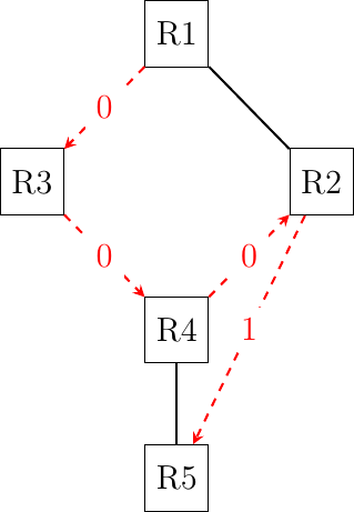
The figure below shows the path followed by the packets on the R1->R3->R4->R2->R5 path in red with on each arrow the label used in the packets.
The path followed by packets for a specific circuit
MultiProtocol Label Switching (MPLS) is the example of a deployed networking technology that relies on label switching. MPLS is more complex than the above description because it has been designed to be easily integrated with datagram technologies. However, the principles remain. Asynchronous Transfer Mode (ATM) and Frame Relay are other examples of technologies that rely on label switching.
Nowadays, most deployed networks rely on distributed algorithms, called routing protocols, to compute the forwarding tables that are installed on the routers. These distributed algorithms are part of the control plane. They are usually implemented in software and are executed on the main CPU of the routers. There are two main families of routing protocols : distance vector routing and link state routing. Both are capable of discovering autonomously the network and react dynamically to topology changes.
Footnotes
- 1
We will see later a more detailed description of Multiprotocol Label Switching, a networking technology that is capable of using one or more labels.
The control plane
One of the objectives of the control plane in the network layer is to maintain the routing tables that are used on all routers. As indicated earlier, a routing table is a data structure that contains, for each destination address (or block of addresses) known by the router, the outgoing interface over which the router must forward a packet destined to this address. The routing table may also contain additional information such as the address of the next router on the path towards the destination or an estimation of the cost of this path.
In this section, we discuss the main techniques that can be used to maintain the forwarding tables in a network.
Distance vector routing
Distance vector routing is a simple distributed routing protocol. Distance vector routing allows routers to automatically discover the destinations reachable inside the network as well as the shortest path to reach each of these destinations. The shortest path is computed based on metrics or costs that are associated to each link. We use l.cost to represent the metric that has been configured for link l on a router.
Each router maintains a routing table. The routing table R can be modeled as a data structure that stores, for each known destination address d, the following attributes :
R[d].link is the outgoing link that the router uses to forward packets towards destination d
R[d].cost is the sum of the metrics of the links that compose the shortest path to reach destination d
R[d].time is the timestamp of the last distance vector containing destination d
A router that uses distance vector routing regularly sends its distance vector over all its interfaces. This distance vector is a summary of the router’s routing table that indicates the distance towards each known destination. This distance vector can be computed from the routing table by using the pseudo-code below.
Every N seconds:
    v = Vector()
    for d in R[]:
        # add destination d to vector
        v.add(Pair(d, R[d].cost))
    for i in interfaces
        # send vector v on this interface
        send(v, i)
When a router boots, it does not know any destination in the network and its routing table only contains its local address(es). It thus sends to all its neighbors a distance vector that contains only its address at a distance of 0. When a router receives a distance vector on link l, it processes it as follows.
# V : received Vector
# l : link over which vector is received
def received(V, l):
    # received vector from link l
    for d in V[]
        if not (d in R[]):
            # new route
            R[d].cost = V[d].cost + l.cost
            R[d].link = l
            R[d].time = now
        else:
            # existing route, is the new better ?
            if ((V[d].cost + l.cost) < R[d].cost) or (R[d].link == l):
                # Better route or change to current route
                R[d].cost = V[d].cost + l.cost
                R[d].link = l
                R[d].time = now
The router iterates over all addresses included in the distance vector. If the distance vector contains a destination address that the router does not know, it inserts it inside its routing table via link l and at a distance which is the sum between the distance indicated in the distance vector and the cost associated to link l. If the destination was already known by the router, it only updates the corresponding entry in its routing table if either :
the cost of the new route is smaller than the cost of the already known route ((V[d].cost + l.cost) < R[d].cost)
the new route was learned over the same link as the current best route towards this destination (R[d].link == l)
The first condition ensures that the router discovers the shortest path towards each destination. The second condition is used to take into account the changes of routes that may occur after a link failure or a change of the metric associated to a link.
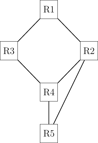
To understand the operation of a distance vector protocol, let us consider the network of five routers shown below.
Operation of distance vector routing in a simple network
Assume that router A is the first to send its distance vector [A=0].
B and D process the received distance vector and update their routing table with a route towards A.
D sends its distance vector [D=0,A=1] to A and E. E can now reach A and D.
C sends its distance vector [C=0] to B and E
E sends its distance vector [E=0,D=1,A=2,C=1] to D, B and C. B can now reach A, C, D and E
B sends its distance vector [B=0,A=1,C=1,D=2,E=1] to A, C and E. A, B, C and E can now reach all five routers of this network.
A sends its distance vector [A=0,B=1,C=2,D=1,E=2] to B and D.
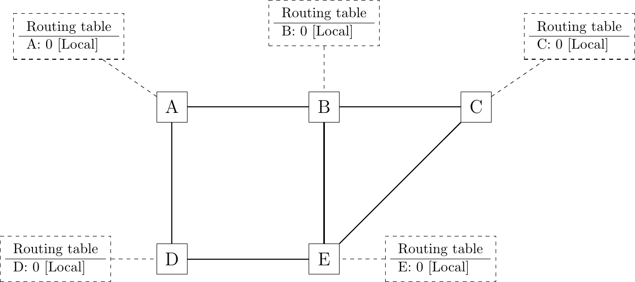
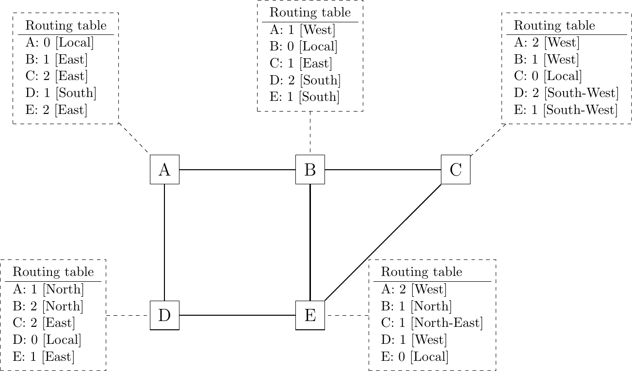
At this point, all routers can reach all other routers in the network thanks to the routing tables shown in the figure below.
Routing tables computed by distance vector in a simple network
To deal with link and router failures, routers use the timestamp stored in their routing table. As all routers send their distance vector every N seconds, the timestamp of each route should be regularly refreshed. Thus no route should have a timestamp older than N seconds, unless the route is not reachable anymore. In practice, to cope with the possible loss of a distance vector due to transmission errors, routers check the timestamp of the routes stored in their routing table every N seconds and remove the routes that are older than \(3 \times N\) seconds.
When a router notices that a route towards a destination has expired, it must first associate an \(\infty\) cost to this route and send its distance vector to its neighbors to inform them. The route can then be removed from the routing table after some time (e.g. \(3 \times N\) seconds), to ensure that the neighboring routers have received the bad news, even if some distance vectors do not reach them due to transmission errors.
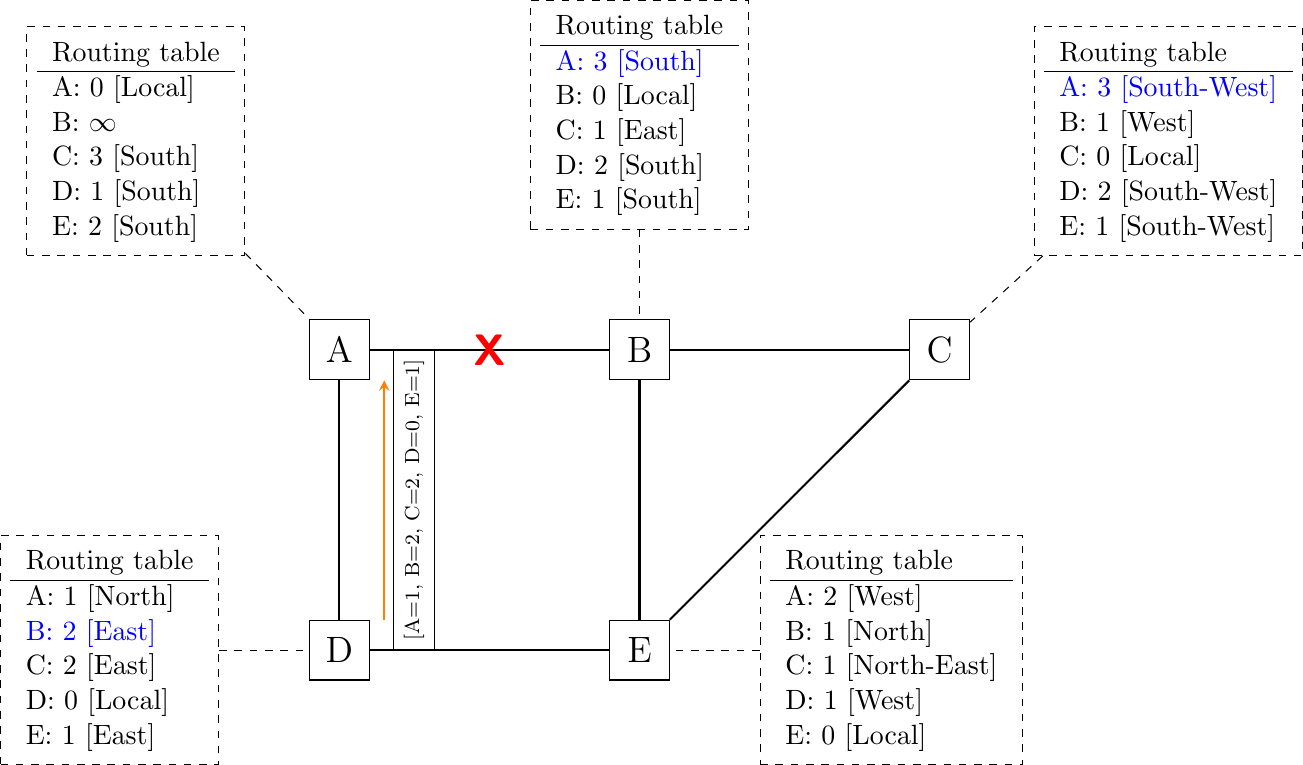
Consider the example above and assume that the link between routers A and B fails. Before the failure, A used B to reach destinations B, C and E while B only used the A-B link to reach A. The two routers detect the failure by the timeouts in the affected entries in their routing tables. Both routers A and B send their distance vector.
A sends its distance vector \([A=0,B=\infty,C=\infty,D=1,E=\infty]\). D knows that it cannot reach B anymore via A
D sends its distance vector \([D=0,B=\infty,A=1,C=2,E=1]\) to A and E. A recovers routes towards C and E via D.
B sends its distance vector \([B=0,A=\infty,C=1,D=2,E=1]\) to E and C. C learns that there is no route anymore to reach A via B.
E sends its distance vector \([E=0,A=2,C=1,D=1,B=1]\) to D, B and C. D learns a route towards B. C and B learn a route towards A.
At this point, all routers have a routing table allowing them to reach all other routers, except router A, which cannot yet reach router B. A recovers the route towards B once router D sends its updated distance vector \([A=1,B=2,C=2,D=0,E=1]\). This last step is illustrated in figure below, which shows the routing tables on all routers.
Routing tables computed by distance vector after a failure
Consider now that the link between D and E fails. The network is now partitioned into two disjoint parts: (A , D) and (B, E, C). The routes towards B, C and E expire first on router D. At this time, router D updates its routing table.
If D sends \([D=0, A=1, B=\infty, C=\infty, E=\infty]\), A learns that B, C and E are unreachable and updates its routing table.
Unfortunately, if the distance vector sent to A is lost or if A sends its own distance vector ( \([A=0,D=1,B=3,C=3,E=2]\) ) at the same time as D sends its distance vector, D updates its routing table to use the shorter routes advertised by A towards B, C and E. After some time D sends a new distance vector : \([D=0,A=1,E=3,C=4,B=4]\). A updates its routing table and after some time sends its own distance vector \([A=0,D=1,B=5,C=5,E=4]\), etc. This problem is known as the count to infinity problem in the networking literature.
Routers A and D exchange distance vectors with increasing costs until these costs reach \(\infty\). This problem may occur in other scenarios than the one depicted in the above figure. In fact, distance vector routing may suffer from count to infinity problems as soon as there is a cycle in the network. Unfortunately, cycles are widely used in networks since they provide the required redundancy to deal with link and router failures. To mitigate the impact of counting to infinity, some distance vector protocols consider that \(16=\infty\). Unfortunately, this limits the metrics that network operators can use and the diameter of the networks using distance vectors.
This count to infinity problem occurs because router A advertises to router D a route that it has learned via router D. A possible solution to avoid this problem could be to change how a router creates its distance vector. Instead of computing one distance vector and sending it to all its neighbors, a router could create a distance vector that is specific to each neighbor and only contains the routes that have not been learned via this neighbor. This could be implemented by the following pseudocode.
# split horizon
Every N seconds:
    # one vector for each interface
    for l in interfaces:
        v = Vector()
        for d in R[]:
            if (R[d].link != l):
                v = v + Pair(d, R[d].cost)
        send(v, l)
        # end for d in R[]
    # end for l in interfaces
This technique is called split-horizon. With this technique, the count to infinity problem would not have happened in the above scenario, as router A would have advertised \([A=0]\) after the failure, since it learned all its other routes via router D. Another variant called split-horizon with poison reverse is also possible. Routers using this variant advertise a cost of \(\infty\) for the destinations that they reach via the router to which they send the distance vector. This can be implemented by using the pseudo-code below.
# split horizon with poison reverse
Every N seconds:
    for l in interfaces:
        # one vector for each interface
        v = Vector()
        for d in R[]:
            if (R[d].link != l):
                v = v + Pair(d, R[d].cost)
            else:
                v = v + Pair(d, infinity)
        send(v, l)
        # end for d in R[]
    # end for l in interfaces
Unfortunately, split-horizon is not sufficient to avoid all count to infinity problems with distance vector routing. Consider the failure of link A-B in the four routers network shown below.
Count to infinity problem
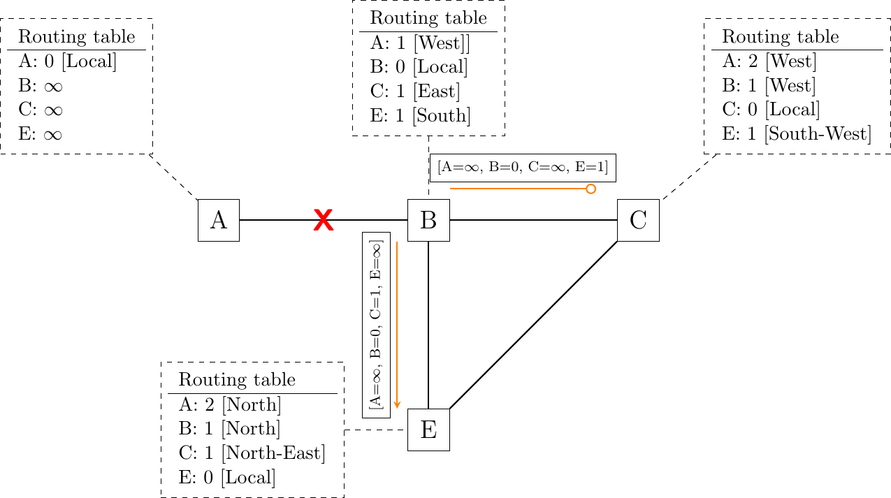
After having detected the failure, router B sends its distance vectors:
\([A=\infty,B=0,C=\infty,E=1]\) to router C
\([A=\infty,B=0,C=1,E=\infty]\) to router E
If, unfortunately, the distance vector sent to router C is lost due to a transmission error or because router C is overloaded, a new count to infinity problem can occur. If router C sends its distance vector \([A=2,B=1,C=0,E=\infty]\) to router E, this router installs a route of distance 3 to reach A via C. Router E sends its distance vectors \([A=3,B=\infty,C=1,E=1]\) to router B and \([A=\infty,B=1,C=\infty,E=0]\) to router C. This distance vector allows B to recover a route of distance 4 to reach A.
Note
Forwarding tables versus routing tables
Routers usually maintain at least two data structures that contain information about the reachable destinations. The first data structure is the routing table. The routing table is a data structure that associates a destination to an outgoing interface or a nexthop router and a set of additional attributes. Different routing protocols can associate different attributes for each destination. Distance vector routing protocols will store the cost to reach the destination along the shortest path. Other routing protocols may store information about the number of hops of the best path, its lifetime or the number of sub paths. A routing table may store different paths towards a given destination and flag one of them as the best one.
The routing table is a software data structure which is updated by (one or more) routing protocols. The routing table is usually not directly used when forwarding packets. Packet forwarding relies on a more compact data structure which is the forwarding table. On high-end routers, the forwarding table is implemented directly in hardware while lower performance routers will use a software implementation. A forwarding table contains a subset of the information found in the routing table. It only contains the nexthops towards each destination that are used to forward packets and no attributes. A forwarding table will typically associate each destination to one or more outgoing interface or nexthop router.
Link state routing
Link state routing is the second family of routing protocols. While distance vector routers use a distributed algorithm to compute their routing tables, link-state routers exchange messages to allow each router to learn the entire network topology. Based on this learned topology, each router is then able to compute its routing table by using a shortest path computation such as Dijkstra’s algorithm [Dijkstra1959]. A detailed description of this shortest path algorithm may be found in [Wikipedia:Dijkstra].
For link-state routing, a network is modeled as a directed weighted graph. Each router is a node, and the links between routers are the edges in the graph. A positive weight is associated to each directed edge and routers use the shortest path to reach each destination. In practice, different types of weights can be associated to each directed edge :
unit weight. If all links have a unit weight, shortest path routing prefers the paths with the least number of intermediate routers.
weight proportional to the propagation delay on the link. If all link weights are configured this way, shortest path routing uses the paths with the smallest propagation delay.
\(weight=\frac{C}{bandwidth}\) where C is a constant larger than the highest link bandwidth in the network. If all link weights are configured this way, shortest path routing prefers higher bandwidth paths over lower bandwidth paths.
Usually, the same weight is associated to the two directed edges that correspond to a physical link (i.e. \(R1 \rightarrow R2\) and \(R2 \rightarrow R1\)). However, nothing in the link state protocols requires this. For example, if the weight is set in function of the link bandwidth, then an asymmetric ADSL link could have a different weight for the upstream and downstream directions. Other variants are possible. Some networks use optimization algorithms to find the best set of weights to minimize congestion inside the network for a given traffic demand [FRT2002].
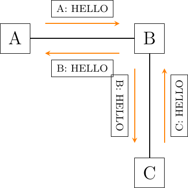
When a link-state router boots, it first needs to discover to which routers it is directly connected. For this, each router sends a HELLO message every N seconds on all its interfaces. This message contains the router’s address. Each router has a unique address. As its neighboring routers also send HELLO messages, the router automatically discovers to which neighbors it is connected. These HELLO messages are only sent to neighbors that are directly connected to a router, and a router never forwards the HELLO messages that it receives. HELLO messages are also used to detect link and router failures. A link is considered to have failed if no HELLO message has been received from a neighboring router for a period of \(k \times N\) seconds.
The exchange of HELLO messages
Once a router has discovered its neighbors, it must reliably distribute all its outgoing edges to all routers in the network to allow them to compute their local view of the network topology. For this, each router builds a link-state packet (LSP) containing the following information:
LSP.Router: identification (address) of the sender of the LSP
LSP.age: age or remaining lifetime of the LSP
LSP.seq: sequence number of the LSP
LSP.Links[]: links advertised in the LSP. Each directed link is represented with the following information:
LSP.Links[i].Id: identification of the neighbor
LSP.Links[i].cost: cost of the link
These LSPs must be reliably distributed inside the network without using the router’s routing table since these tables can only be computed once the LSPs have been received. The Flooding algorithm is used to efficiently distribute the LSPs of all routers. Each router that implements flooding maintains a link state database (LSDB) containing the most recent LSP sent by each router. When a router receives a LSP, it first verifies whether this LSP is already stored inside its LSDB. If so, the router has already distributed the LSP earlier and it does not need to forward it. Otherwise, the router forwards the LSP on all its links except the link over which the LSP was received. Flooding can be implemented by using the following pseudo-code.
# links is the set of all links on the router
# Router R's LSP arrival on link l
if newer(LSP, LSDB(LSP.Router)) :
    LSDB.add(LSP)  # implicitly removes older LSP from same router
    for i in links:
        if i!=l:
           send(LSP,i)
# else, LSP has already been flooded
In this pseudo-code, LSDB(r) returns the most recent LSP originating from router r that is stored in the LSDB. newer(lsp1, lsp2) returns true if lsp1 is more recent than lsp2. See the note below for a discussion on how newer can be implemented.
Note
Which is the most recent LSP ?
A router that implements flooding must be able to detect whether a received LSP is newer than the stored LSP. This requires a comparison between the sequence number of the received LSP and the sequence number of the LSP stored in the link state database. The ARPANET routing protocol [MRR1979] used a 6 bits sequence number and implemented the comparison as follows RFC 789
def newer( lsp1, lsp2 ):
    return ( ((lsp1.seq > lsp2.seq) and ((lsp1.seq - lsp2.seq) <= 32)) or
           ( (lsp1.seq < lsp2.seq) and ((lsp2.seq - lsp1.seq) > 32)) )
This comparison takes into account the modulo \(2^{6}\) arithmetic used to increment the sequence numbers. Intuitively, the comparison divides the circle of all sequence numbers into two halves. Usually, the sequence number of the received LSP is equal to the sequence number of the stored LSP incremented by one, but sometimes the sequence numbers of two successive LSPs may differ, e.g. if one router has been disconnected for some time. The comparison above worked well until October 27, 1980. On this day, the ARPANET crashed completely. The crash was complex and involved several routers. At one point, LSP 40 and LSP 44 from one of the routers were stored in the LSDB of some routers in the ARPANET. As LSP 44 was the newest, it should have replaced LSP 40 on all routers. Unfortunately, one of the ARPANET routers suffered from a memory problem and sequence number 40 (101000 in binary) was replaced by 8 (001000 in binary) in the buggy router and flooded. Three LSPs were present in the network and 44 was newer than 40 which is newer than 8, but unfortunately 8 was considered to be newer than 44… All routers started to exchange these three link state packets forever and the only solution to recover from this problem was to shutdown the entire network RFC 789.
Current link state routing protocols usually use 32 bits sequence numbers and include a special mechanism in the unlikely case that a sequence number reaches the maximum value (with a 32 bits sequence number space, it takes 136 years to cycle the sequence numbers if a link state packet is generated every second).
To deal with the memory corruption problem, link state packets contain a checksum or CRC. This checksum is computed by the router that generates the LSP. Each router must verify the checksum when it receives or floods an LSP. Furthermore, each router must periodically verify the checksums of the LSPs stored in its LSDB. This enables them to cope with memory errors that could corrupt the LSDB as the one that occurred in the ARPANET.
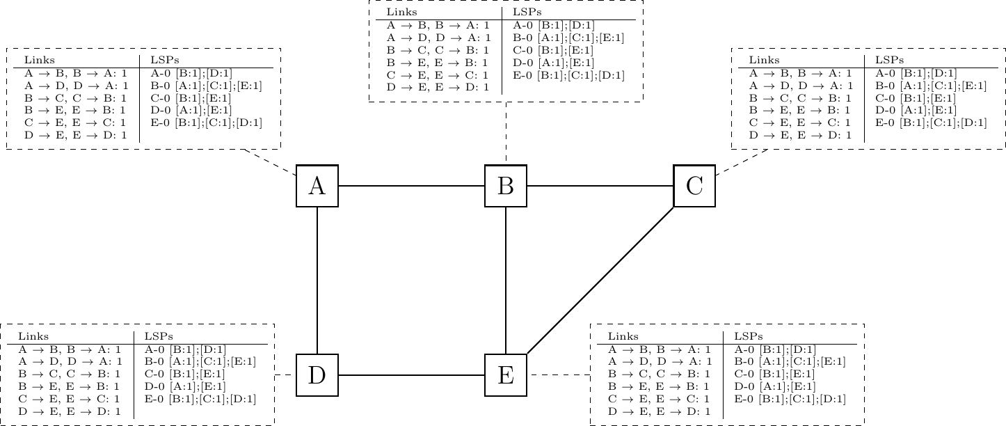
Flooding is illustrated in the figure below. By exchanging HELLO messages, each router learns its direct neighbors. For example, router E learns that it is directly connected to routers D, B and C. Its first LSP has sequence number 0 and contains the directed links E->D, E->B and E->C. Router E sends its LSP on all its links and routers D, B and C insert the LSP in their LSDB and forward it over their other links.
Flooding: example
Flooding allows LSPs to be distributed to all routers inside the network without relying on routing tables. In the example above, the LSP sent by router E is likely to be sent twice on some links in the network. For example, routers B and C receive E’s LSP at almost the same time and forward it over the B-C link. To avoid sending the same LSP twice on each link, a possible solution is to slightly change the pseudo-code above so that a router waits for some random time before forwarding a LSP on each link. The drawback of this solution is that the delay to flood an LSP to all routers in the network increases. In practice, routers immediately flood the LSPs that contain new information (e.g. addition or removal of a link) and delay the flooding of refresh LSPs (i.e. LSPs that contain exactly the same information as the previous LSP originating from this router) [FFEB2005].
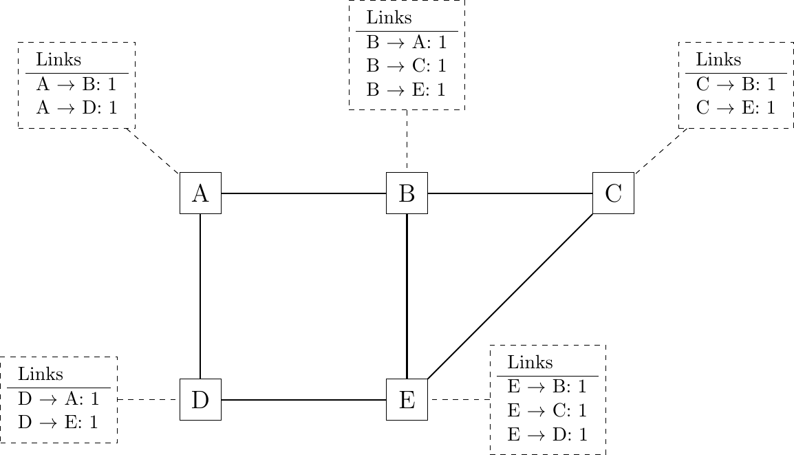
To ensure that all routers receive all LSPs, even when there are transmissions errors, link state routing protocols use reliable flooding. With reliable flooding, routers use acknowledgments and if necessary retransmissions to ensure that all link state packets are successfully transferred to each neighboring router. Thanks to reliable flooding, all routers store in their LSDB the most recent LSP sent by each router in the network. By combining the received LSPs with its own LSP, each router can build a graph that represents the entire network topology.
Link state databases received by all routers
Note
Static or dynamic link metrics ?
As link state packets are flooded regularly, routers are able to measure the quality (e.g. delay or load) of their links and adjust the metric of each link according to its current quality. Such dynamic adjustments were included in the ARPANET routing protocol [MRR1979] . However, experience showed that it was difficult to tune the dynamic adjustments and ensure that no forwarding loops occur in the network [KZ1989]. Today’s link state routing protocols use metrics that are manually configured on the routers and are only changed by the network operators or network management tools [FRT2002].
When a link fails, the two routers attached to the link detect the failure by the absence of HELLO messages received during the last \(k \times N\) seconds. Once a router has detected the failure of one of its local links, it generates and floods a new LSP that no longer contains the failed link. This new LSP replaces the previous LSP in the network. In practice, the two routers attached to a link do not detect this failure exactly at the same time. During this period, some links may be announced in only one direction. This is illustrated in the figure below. Router E has detected the failure of link E-B and flooded a new LSP, but router B has not yet detected this failure.
The two-way connectivity check
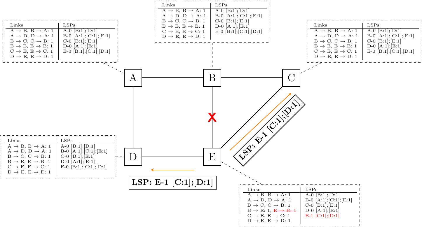
When a link is reported in the LSP of only one of the attached routers, routers consider the link as having failed and they remove it from the directed graph that they compute from their LSDB. This is called the two-way connectivity check. This check allows link failures to be quickly flooded as a single LSP is sufficient to announce such bad news. However, when a link comes up, it can only be used once the two attached routers have sent their LSPs. The two-way connectivity check also allows for dealing with router failures. When a router fails, all its links fail by definition. These failures are reported in the LSPs sent by the neighbors of the failed router. The failed router does not, of course, send a new LSP to announce its failure. However, in the graph that represents the network, this failed router appears as a node that only has outgoing edges. Thanks to the two-way connectivity check, this failed router cannot be considered as a transit router to reach any destination since no outgoing edge is attached to it.
When a router has failed, its LSP must be removed from the LSDB of all routers 2. This can be done by using the age field that is included in each LSP. The age field is used to bound the maximum lifetime of a link state packet in the network. When a router generates a LSP, it sets its lifetime (usually measured in seconds) in the age field. All routers regularly decrement the age of the LSPs in their LSDB and a LSP is discarded once its age reaches 0. Thanks to the age field, the LSP from a failed router does not remain in the LSDBs forever.
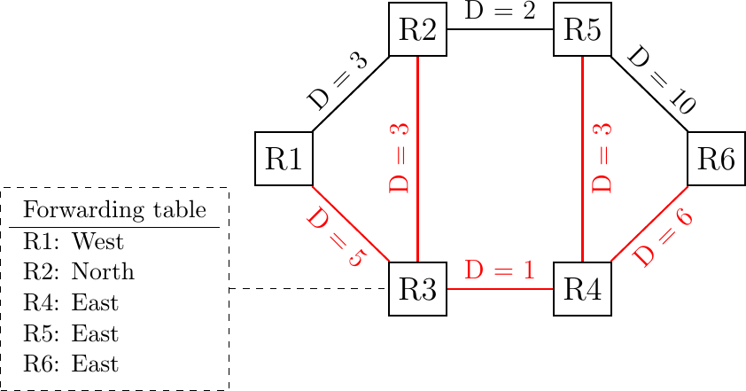
To compute its forwarding table, each router computes the spanning tree rooted at itself by using Dijkstra’s shortest path algorithm [Dijkstra1959]. The forwarding table can be derived automatically from the spanning as shown in the figure below.
Computation of the forwarding table, the paths used by packets sent by R3 are shown in red
Footnotes
- 2
It should be noted that link state routing assumes that all routers in the network have enough memory to store the entire LSDB. The routers that do not have enough memory to store the entire LSDB cannot participate in link state routing. Some link state routing protocols allow routers to report that they do not have enough memory and must be removed from the graph by the other routers in the network, but this is outside the scope of this e-book.